Comparing Excel sheets is a common task in data management, yet it often becomes tedious without the right approach. My Online Training Hub explores three practical methods to simplify this process, including a lesser-known technique for advanced users. For instance, using Excel’s “New Window” and “Arrange All” features allows you to view two sheets side-by-side, creating a clear visual comparison. This foundational step not only minimizes errors but also sets the stage for more detailed methods like formula-based checks or Power Query integrations.
In this breakdown, you’ll uncover how to use conditional formatting to highlight mismatched data, create an audit sheet for systematic comparisons and apply Power Query for handling large or complex datasets. Each method is tailored to specific scenarios, from quick checks to in-depth audits, making sure you can adapt to your data needs. Whether you’re reconciling financial records or tracking project updates, these techniques offer actionable ways to enhance accuracy and efficiency.
Set Up Your Workspace for Efficiency
TL;DR Key Takeaways :
- Prepare your workspace by using Excel’s “New Window” and “Arrange All” features to view sheets side-by-side for easier comparison.
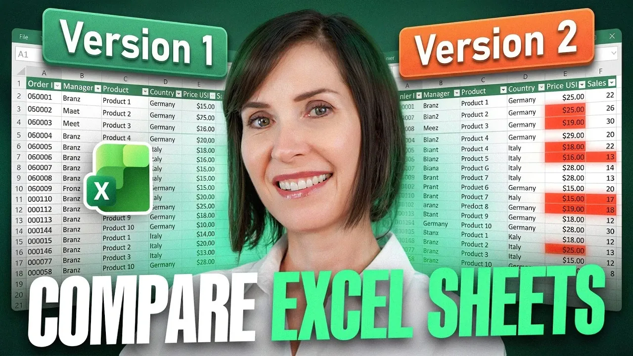
- Use Conditional Formatting to visually highlight differences between sheets, ideal for smaller datasets or quick checks.
- Create an Audit Sheet for structured comparisons, using formulas to systematically identify and document discrepancies.
- Use Power Query for advanced comparisons, especially for large or complex datasets with added, removed, or reordered rows.
- Address common issues like trailing spaces, numbers stored as text and date inconsistencies to ensure accurate and reliable comparisons.
Before diving into specific comparison methods, it’s crucial to prepare your workspace for optimal efficiency. Excel’s built-in features, such as “New Window” and “Arrange All,” allow you to view two sheets side-by-side, making it easier to identify discrepancies without switching between tabs.
To set up your workspace:
- Open the workbook(s) containing the sheets you want to compare.
- Go to the View tab in the ribbon and click New Window to open a duplicate view of your workbook.
- Select Arrange All and choose a layout, such as “Vertical” or “Horizontal,” to display the sheets side-by-side.
This setup provides a clear visual comparison, laying the groundwork for more detailed methods. It’s a simple yet effective way to streamline your workflow and reduce errors.
Method 1: Conditional Formatting
Conditional formatting is a straightforward way to visually highlight differences between two sheets. By applying a formula-based rule, you can quickly identify mismatched cells, making this method ideal for smaller datasets or quick checks.
Steps to apply conditional formatting:
- Select the range of cells in the first sheet that you want to compare.
- Navigate to Home > Conditional Formatting > New Rule.
- Choose “Use a formula to determine which cells to format.”
- Enter a formula such as
=A1<>Sheet2!A1, adjusting the cell references to match your dataset.
This method is particularly effective for identifying:
- Trailing spaces: Use the LEN function to detect extra spaces that may cause cells to appear identical but differ in content.
- Numbers stored as text: Resolve these inconsistencies using Excel’s error-checking tools or by converting text to numbers.
- Date formatting mismatches: Standardize date formats to ensure consistency across sheets.
While conditional formatting is user-friendly and visually intuitive, it may not be suitable for large datasets or scenarios involving structural changes, such as added or deleted rows.

Here is a selection of other guides from our extensive library of content you may find of interest on Excel.
- Excel with Claude: Pre-Built Skills for DCF and Comps Save Hours
- Claude in Excel vs Copilot : Strengths & Weaknesses Tested
- How to convert a PDF file to Excel without software
- Zero-Click Excel Automation in Microsoft 365 with Scripts
- How to Unprotect an Excel Sheet Without a Password
- 10 Essential Excel Formula Symbols to Boost Your Productivity
- 12 Apple Numbers Features That Outshine Excel in 2025
- Microsoft Copilot 2026 Tutorial for Excel, PowerPoint, Teams, Outlook
- Master Advanced Excel Functions BYROW vs MAP vs SCAN vs REDUCE
- 14 New Microsoft Excel Features for Fall 2024 You Should Know
Method 2: Create an Audit Sheet
For a more structured and detailed approach, creating an audit sheet is highly effective. This method involves building a third sheet that systematically identifies and displays differences between the two sheets.
Steps to create an audit sheet:
- Add a new sheet to your workbook and label it clearly, such as “Audit Sheet.”
- Use an IF formula to compare cells. For example, enter
=IF(Sheet1!A1=Sheet2!A1, "Match", "Mismatch")in a cell and drag it across the relevant range. - Organize the results with clear column headers, such as “Sheet1 Value,” “Sheet2 Value,” and “Comparison Result.”
This method is particularly useful for audits or reporting, as it provides a clear and systematic record of discrepancies. You can also customize the formulas to flag specific issues, such as “Value Changed” or “Data Missing.” The audit sheet serves as a reliable reference for stakeholders or team members, making sure transparency and accuracy.
Method 3: Power Query for Advanced Comparisons
For large or complex datasets, Power Query offers a robust solution. Unlike cell-by-cell comparisons, Power Query operates at the row level, making it ideal for scenarios where rows have been added, removed, or reordered.
Steps to use Power Query:
- Format your data as tables in both sheets by selecting the range and clicking Insert > Table.
- Load the tables into Power Query by selecting Data > Get & Transform > From Table/Range.
- Use the Merge Queries option to combine the tables. For example, select “Left Anti Join” to identify rows that exist in one table but not the other.
Power Query dynamically updates its results when the data changes, making it a time-saving tool for recurring tasks or large datasets. Its flexibility and scalability make it an indispensable option for advanced users handling complex data comparisons.
Common Issues and How to Fix Them
When comparing Excel sheets, you may encounter common challenges that can affect accuracy. Addressing these issues ensures reliable results:
- Trailing spaces: Use the TRIM function to remove unnecessary spaces that can cause false mismatches.
- Numbers stored as text: Convert these using Excel’s error-checking tools or the VALUE function to standardize data types.
- Date inconsistencies: Standardize date formats by selecting Home > Number Format > Short Date or applying a custom format.
By resolving these issues, you can prevent errors and ensure that your comparisons are both accurate and meaningful.
Practical Applications
The methods outlined here are versatile and applicable to a wide range of scenarios:
- Data auditing: Quickly identify and resolve discrepancies in financial records, inventory lists, or other datasets.
- Change tracking: Generate detailed reports for stakeholders, highlighting updates or errors in your data.
- Automation: Use Power Query for scalable, repeatable comparisons, especially in large or frequently updated datasets.
By mastering these techniques, you can streamline your workflow, reduce errors and gain deeper insights into your data. Whether you’re working with small spreadsheets or extensive databases, these methods provide reliable tools for efficient and accurate comparisons.
Media Credit: MyOnlineTrainingHub
Disclosure: Some of our articles include affiliate links. If you buy something through one of these links, Geeky Gadgets may earn an affiliate commission. Learn about our Disclosure Policy.